In 2015, we published ExSTraCS 2.0 and reported that we had successfully solved the 135 bit Multiplexer problem (Figure 1). This is the first, and to date, only time an algorithm has reported solving this complex benchmark data science problem directly. Additionally we solved this problem in a way that makes the problem particularly challenging (i.e. only being able to learn on a finite sampling of training instances from the problem space. Below we explain the Multiplexer problem and why it is important and interesting as a benchmark. The Multiplexer problem reflects properties that are relevant to challenges within complex real world problems, such as bioinformatics, finance, and behavior modeling. Keep in mind that this benchmark problem alone does not capture the full range of applications to which a Learning Classifier System or ExSTraCS is capable.
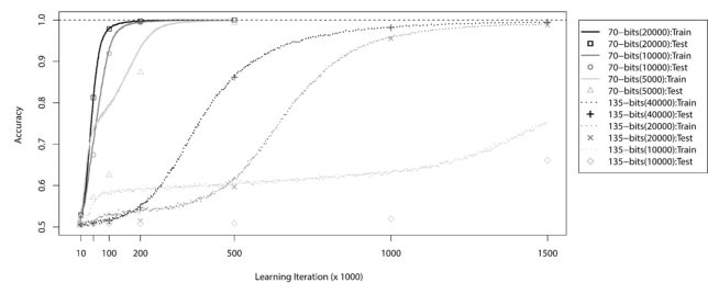
Figure 1: ExSTraCS 2.0 solving the 70-bit and 135-bit Multiplexer problems with different training sample sizes.
The Boolean n-bit Multiplexer defines a set of single-step supervised learning problems (e.g. 6-bit, 11-bit) that are conceptually based on the behavior of an electronic multiplexer (MUX), a device that takes multiple analog or digital input signals and switches them into a single output. The 6-bit multiplexer problem, is illustrated in Figure 2. To generate a 6-bit multiplexer training dataset we can generate random bit-strings of length six and for each, the class/output value is determined by the two address bits and the value at the register bit they point to. In Figure ?? we see that the first instance from the training data has the bit-string state of `010110′. Each binary digit represents a distinct feature in the dataset that can have one of two values `0′ or `1′. Features can also be referred to as attributes, or independent variables. In the 6-bit multiplexer problem, the first two features are address bits. The address `01′ points to the register bit with ID = 1 (i.e. the second register bit). The value of that register bit equals 1, thus the class of this instance equals 1. The class of an instance can also be referred to as the endpoint, action, phenotype, or dependant variable based on the problem at hand. If you examine other example instances from the training data in Figure 2 you can verify this relationship between address and register bits. Since the 6-bit multiplexer has 2 address bits and 4 register bits, it has also been referred to as the 2-4 multiplexer problem.
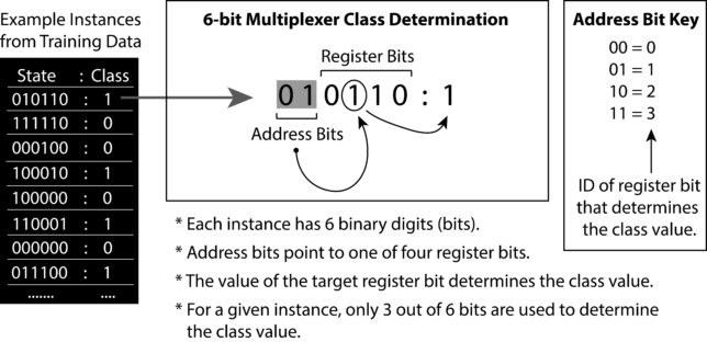
Figure 2: Example instances and description of the 6-bit multiplexer problem (taken from “Introduction to LCS” textbook).
Any multiplexer problem is non-trivial because it relies on a fairly complicated pattern to determine class. John Koza, best known for his work pioneering genetic programming (an evolutionary computation strategy) once wrote; “Multiplexer functions have long been identified by researchers as functions that often pose difficulties for paradigms for machine learning, artificial intelligence, neural nets, and classifier systems.” In particular every multiplexer problem involves an interaction effect between multiple features, also known as epistasis. They also exhibit heterogeneity, where for different sets of instances, a distinct subset of features will determine the class value. An association between a single variable and an endpoint of interest can be referred to as a main effect, or a linear association. Most machine learning algorithms, including LCS, are proficient at detecting linear relationships. Notice that in multiplexer problems, knowing the value of any single bit/feature alone provides no information about class. For example, in the 6-bit problem, while class is directly based on the value of one of the register bits, we must also identify the states of the two address bits to know which register bit to pay attention to. While some machine learning algorithms (e.g. genetic programming, and artificial neural networks), are able to automatically model epistatic interactions, LCS algorithms are uniquely suited to the complexities of both epistasis and heterogeneity. Indeed, multiplexer problems have been an important and defining benchmark for LCS algorithms for many years. While the multiplexer problems themselves are ‘toy’ benchmark problems, their characteristic patterns of epistasis and heterogeneity are directly relatable to real world problems. LCSs have been shown to have the ability to detect these types of complex patterns in real world problems, where noise and a lack of prior knowledge about the problem domain further complicate these tasks.
Conveniently, the n-bit Multiplexer can be scaled up in complexity by simply increasing the number of address bits from two, upwards. The table below details the set of multiplexer problems that have been successfully solved by an LCS algorithm without any prior problem domain knowledge. The `order of interaction’ refers to the number of features that interact to determine class within a given instance (i.e. epistasis). The `heterogeneous combinations’ refers to the number of distinct feature subsets that must be identified in order to solve the problem completely (and conveniently this column also gives the correct number of register bits). Each heterogeneous feature subset in a multiplexer problem has the corresponding order of interaction. In other words, for the 6-bit multiplexer, LCS must find 4 unique combinations of 3-feature subsets in order to completely solve the problem. `Unique instances’ gives the total number of unique training instances that are possible, and `optimal rules’ gives the minimum number of optimal rules required for an LCS algorithm to completely solve the corresponding problem. Be aware that this calculation of the number of optimal rules is based on two assumptions; (1) that we have employed the ternary rule representation, and (2) we are searching for a best action map. Therefore, other LCS implementations can yield a different number of optimal rules.
The optimal rules each cover different niches in the problem space of the 6-bit multiplexer problem. These niches are identified by the different colors in Figure 3.
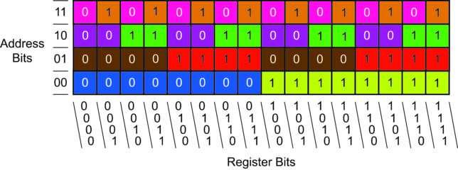
Figure 3: Niches covered by `optimal rules’ in the 6-bit Multiplexer problem.